

Study with the several resources on Docsity
Earn points by helping other students or get them with a premium plan
Prepare for your exams
Study with the several resources on Docsity
Earn points to download
Earn points by helping other students or get them with a premium plan
Community
Ask the community for help and clear up your study doubts
Discover the best universities in your country according to Docsity users
Free resources
Download our free guides on studying techniques, anxiety management strategies, and thesis advice from Docsity tutors
Material Type: Assignment; Class: 670 - REM SENS OCEAN+ATMOS; Subject: METEOROLOGY; University: Rutgers University; Term: Spring 2008;
Typology: Assignments
1 / 3
This page cannot be seen from the preview
Don't miss anything!
11:670:451 / 16:712:552 Remote Sensing of the Ocean and Atmosphere
Homework 4
Due Wednesday April 16, 2008
To distinguish 3 cm of sea level variability with pulse-limited altimetry, the radar pulse itself must be of order 3 cm length. If the pulse duration is T, its length is L = T/c where c is the speed of light. Therefore we need an effective pulse duration of T = L/c = 0.03/3x10^8 = 10-10^ seconds = 0.1 nanoseconds.
In practice, the pulse duration is longer than this and signal compression techniques are applied in the signal processing to deduce the travel time of an “effective pulse” of order this duration.
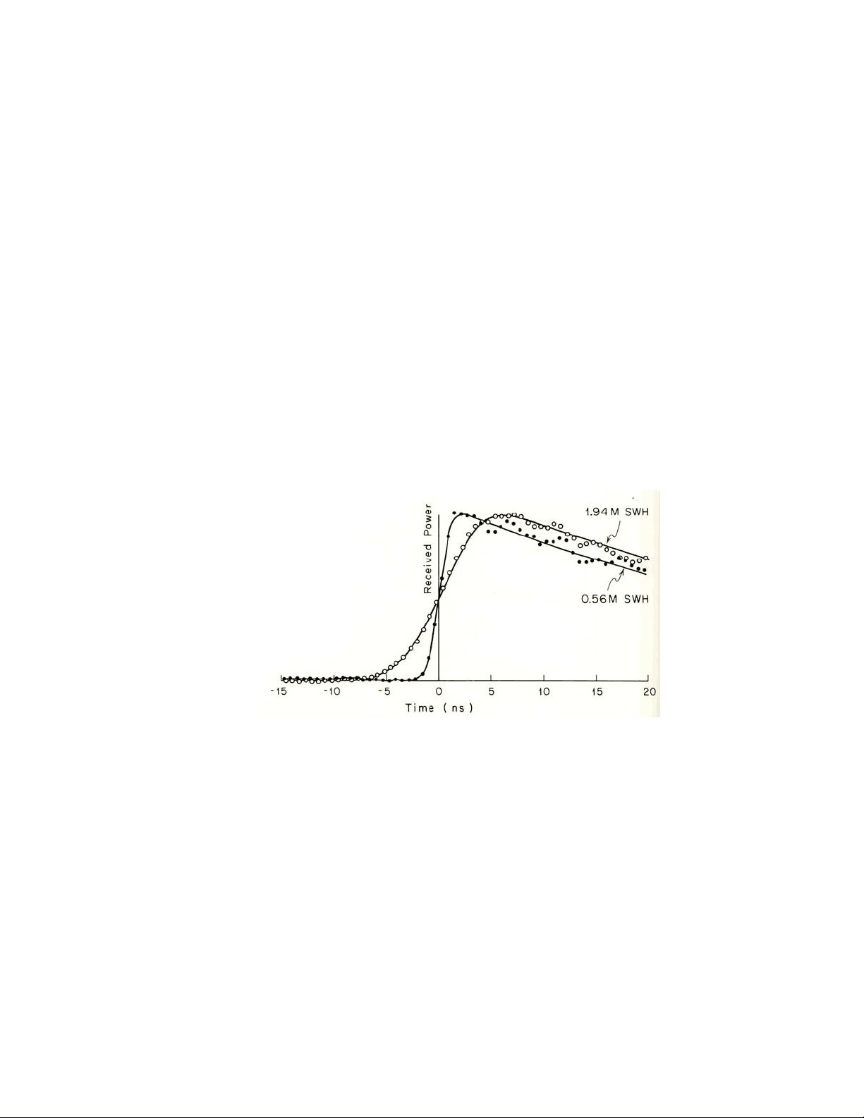
At high SWF the radar return begins early because the wave crests are closer to the satellite, and the return lasts longer because the wave troughs are further from the satellite. Hence, the returned power is stretched out over a greater time interval when wave height is higher.
The number of free electrons in the ionosphere affects the radar pulse transmission time. Electron content varies from day to night (fewer free electrons at night), from summer to winter (fewer during summer), and as a function of the solar cycle (fewer during the solar minimum). This information is obtained by an analysis of travel time variability for transmissions of GPS satellite signals, and in the case of the Poseidon altimeter the transmission of dual-frequency pulses gives a differential response related
to the required ionospheric correction.
Altimeter precision is affected by the speed of light through the troposphere which is affected by (i) the mass of the atmosphere (which is related to the weight of the atmosphere and therefore sea level air pressure) and (ii) the water vapor effect on index of refraction.
(i) is estimated from numerical weather prediction models of MSL pressure.
(ii) is estimated by an onboard radiometer that profiles tropospheric water vapor content, and/or by independent estimates of troposphere water vapor content from atmospheric circulation models (including ECMWF and NCEP).
Sun-synchronous orbits pass over the same point on earth at the same local time, and therefore alias diurnal tides (e.g. S 2 ) with period 12 or 24 hours into zero frequency (i.e. the long term time mean).
A physically large radar antenna can better resolve small angles in directional response. It is impractical to deploy physically large antennas on satellites, but an equivalent performance can be “synthesized” by processing the signals received by a moving antenna as if it were the numerous elements of a large stationary antenna.
a. Range observation
The distance from satellite to sea surface corrected for ionospheric and tropospheric effects on the speed of the radar pluse, and corrected for sea state effects (significant wave height, sea state bias and skewness).
b. Geoid
The geopotential surface corresponding to a stationary ocean.
c. Dynamic topography
The difference between the sea surface height and the geoid due to the dynamics of oceanic circulation. Where the slope of the dynamic topography and slope of the